Data Challenge Lab Home
Spatial basics [wrangle]
(Builds on: Manipulation basics)
(Leads to: Spatial visualization)
Spatial packages
In R, there are two main lineages of tools for dealing with spatial data: sp and sf.
-
sp has been around for a while (the first release was in 2005), and it has a rich ecosystem of tools built on top of it. However, it uses a rather complex data structure, which can make it challenging to use.
-
sf is newer (first released in October 2016) so it doesn’t have such a rich ecosystem. However, it’s much easier to use and fits in very naturally with the tidyverse.
There’s a lot you can do with the sf package, and it contains many more functions that we can cover in this reading. The sf package reference page lists all of the functions in the package. There are also some helpful articles on the package website, including Simple Features for R and Manipulating Simple Feature Geometries.
Loading data
To read spatial data in R, use read_sf(). The following code reads an
example dataset built into the sf package.
library(tidyverse)
library(sf)

# The counties of North Carolina
nc <- read_sf(system.file("shape/nc.shp", package = "sf"))
Here, read_sf() reads from a shapefile. Shapefiles are the most
common way to store spatial data. Despite the name, a shapefile is
actually a collection of files, not a single file. Each file in a
shapefile has the same name, but a different extension. Typically,
you’ll see four files:
-
.shpcontains the geometry -
.shxcontains an index into that geometry. -
.dbfcontains metadata about each geometry (the other columns in the data frame). -
.prfcontains the coordinate system and projection information. You’ll learn more about that shortly.
read_sf() can read in the majority of spatial file formats, and can
likely handle your data even if it isn’t in a shapefile.
Data structure
read_sf() reads in spatial data and creates a tibble, so nc is a
tibble.
class(nc)
#> [1] "sf"         "tbl_df"     "tbl"        "data.frame"
nc functions like an ordinary tibble with one exception: the
geometry column.
nc %>%
  select(geometry)
#> Simple feature collection with 100 features and 0 fields
#> geometry type:  MULTIPOLYGON
#> dimension:      XY
#> bbox:           xmin: -84.32385 ymin: 33.88199 xmax: -75.45698 ymax: 36.58965
#> epsg (SRID):    4267
#> proj4string:    +proj=longlat +datum=NAD27 +no_defs
#> First 10 features:
#>                          geometry
#> 1  MULTIPOLYGON (((-81.47276 3...
#> 2  MULTIPOLYGON (((-81.23989 3...
#> 3  MULTIPOLYGON (((-80.45634 3...
#> 4  MULTIPOLYGON (((-76.00897 3...
#> 5  MULTIPOLYGON (((-77.21767 3...
#> 6  MULTIPOLYGON (((-76.74506 3...
#> 7  MULTIPOLYGON (((-76.00897 3...
#> 8  MULTIPOLYGON (((-76.56251 3...
#> 9  MULTIPOLYGON (((-78.30876 3...
#> 10 MULTIPOLYGON (((-80.02567 3...
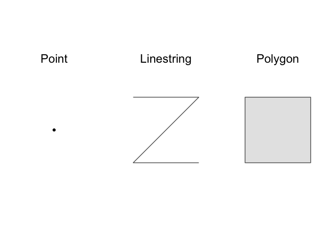
The geometry column contains simple features. Simple features are
a standard way of representing geometry types. The most basic geometry
types are point, linestring, and polygon.
There are also multi variants of these basic types: multipoint, multilinestring, and multipolygon. These multi types can contain multiple points, linestrings, or polygons. The final type, geometry collection, can contain multiple different types (e.g., points, linestrings, and multipolygons).
You can build up complex spatial visualizations using just these geometry types. A point, for example, could represent a city, a multilinestring could represent a branching river, and a multipolygon could represent a country composed of different islands.
nc’s geometry column contains multipolygons.
nc$geometry
#> Geometry set for 100 features
#> geometry type:  MULTIPOLYGON
#> dimension:      XY
#> bbox:           xmin: -84.32385 ymin: 33.88199 xmax: -75.45698 ymax: 36.58965
#> epsg (SRID):    4267
#> proj4string:    +proj=longlat +datum=NAD27 +no_defs
#> First 5 geometries:
#> MULTIPOLYGON (((-81.47276 36.23436, -81.54084 3...
#> MULTIPOLYGON (((-81.23989 36.36536, -81.24069 3...
#> MULTIPOLYGON (((-80.45634 36.24256, -80.47639 3...
#> MULTIPOLYGON (((-76.00897 36.3196, -76.01735 36...
#> MULTIPOLYGON (((-77.21767 36.24098, -77.23461 3...
You can use plot() to visualize the geometry column.
plot(nc$geometry)
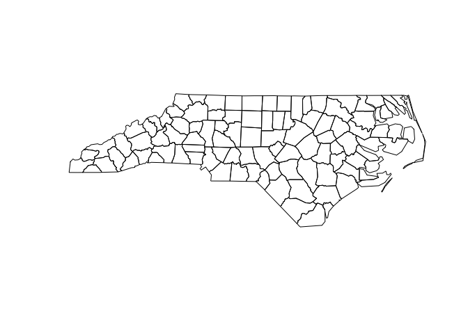
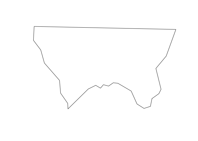
Each row in nc represents a single county. If you pull out a single
row and plot, you’ll get the shape of a single county.
alleghany <-
  nc %>%
  filter(NAME == "Alleghany")

plot(alleghany$geometry)
plot() works, but is limited. In the next unit, you’ll learn how to
use ggplot2 to create more complex spatial visualizations.
Geometry
Let’s dive a little deeper into the structure of the geometry column.
The geometry column is a list-column. You’re used to working with
tibble columns that are atomic vectors, but columns can also be lists.
List columns are incredibly flexible because a list can contain any
other type of data structure, including other lists.
typeof(nc$geometry)
#> [1] "list"
Let’s pull out one row of the geometry column so you can see what’s
going on under the hood.
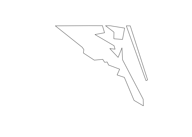
currituck <-
  nc %>%
  filter(NAME == "Currituck")

currituck_geometry <- currituck$geometry[[1]]
Currituck county is made up of three separate landmasses.
plot(currituck_geometry)
How does a single row of the geometry column represent these three
separate shapes? It turns out that each element of nc’s geometry
column, including currituck$geometry, is actually a list of lists of
matrices.
glimpse(currituck_geometry)
#> List of 3
#>  $ :List of 1
#>   ..$ : num [1:26, 1:2] -76 -76 -76 -76 -76.1 ...
#>  $ :List of 1
#>   ..$ : num [1:7, 1:2] -76 -76 -75.9 -75.9 -76 ...
#>  $ :List of 1
#>   ..$ : num [1:5, 1:2] -75.9 -75.9 -75.8 -75.8 -75.9 ...
#>  - attr(*, "class")= chr [1:3] "XY" "MULTIPOLYGON" "sfg"
The top-level list represents landmasses, and has one element for each landmass in the county. Currituck county has three landmasses, and so has three sub-lists.
In our data, each of these sub-lists only has a single element.
map_int(currituck_geometry, length)
#> [1] 1 1 1
These sub-lists would contain multiple elements if they needed to represent a landmass that contained an lake, or a landmass that contained a lake with an island, etc.
Each of these elements is a matrix that gives the locations of points along the polygon boundaries.
currituck_geometry[[2]][[1]]
#>           [,1]     [,2]
#> [1,] -76.02717 36.55672
#> [2,] -75.99866 36.55665
#> [3,] -75.91192 36.54253
#> [4,] -75.92480 36.47398
#> [5,] -75.97728 36.47802
#> [6,] -75.97629 36.51793
#> [7,] -76.02717 36.55672
Manipulating with dplyr
sf objects like nc are tibbles, so you can manipulate them with dplyr.
The following code finds all counties in North Carolina with an area
greater than 2 billion square meters.
nc_large <-
  nc %>%
  mutate(area = st_area(geometry) %>% as.double()) %>%
  filter(area > 2e9)
st_area finds the area of a geometry, and returns an object with
units, in this case square meters.
alleghany %>%
  st_area(geometry)
#> 611077263 [m^2]
These units are helpful, but can be annoying to work with, which is why
we used as.double() in the earlier mutate() statement. as.double()
converts the results to a regular double vector.
The sf package contains many helpful functions, like st_area(), for
working with spatial data. Its reference
page lists all
functions in the package.
Coordinate reference system
Earlier, you saw the following matrix.
currituck_geometry[[2]][[1]]
#>           [,1]     [,2]
#> [1,] -76.02717 36.55672
#> [2,] -75.99866 36.55665
#> [3,] -75.91192 36.54253
#> [4,] -75.92480 36.47398
#> [5,] -75.97728 36.47802
#> [6,] -75.97629 36.51793
#> [7,] -76.02717 36.55672
This matrix gives the position of points along the boundary of one of Currituck county’s landmasses. Geospatial data represents points on the earth in terms of longitude and latitude with respect to a datum. The same point can have a different longitude and latitude with respect to different datums.
Take two minutes and watch this simple explanation of datums.
A coordinate reference system (CRS) for a geospatial dataset
consists of a datum together with a projection that specifies how
points in three dimensions will be represented in two. We can use
st_crs() to find the datum and projection of our data.
st_crs(nc)
#> Coordinate Reference System:
#>   EPSG: 4267
#>   proj4string: "+proj=longlat +datum=NAD27 +no_defs"
The datum of nc is “NAD27”, the North American
Datum of 1927
(NAD27). And the projection is to simply use the longitude and latitude.
When plotting multiple datasets, it is important that they all use the
same CRS. Otherwise, points won’t properly line up. Fortunately,
st_transform() can be used to transform datasets to a common CRS, and
ggplot2 will automatically convert layers to have a common CRS.