Manipulation basics [wrangle]

(Builds on: Data basics)
(Leads to: Data structure basics, Exploratory data analysis (1D), Vector functions, Other single-table verbs, Scoped verb basics, Parsing basics, Spatial basics)

library(tidyverse)
library(nycflights13)

dplyr basics

In this reading you will going to learn about three important dplyr functions that give you basic data manipulation power:

Pick observations by their values (filter()).
Create new variables with functions of existing variables (mutate()).
Collapse many values down to a single summary (summarize()).

These can all be used in conjunction with group_by() which changes the scope of each function from operating on the entire dataset to operating on it group-by-group.

(Use the data transformation cheatsheet to jog your memory, and learn about other dplyr functions we’ll cover in the future)

All dplyr verbs work similarly:

The first argument is a data frame.
The subsequent arguments describe what to do with the data frame.
The result is a new data frame.

Together these properties make it easy to chain together multiple simple steps to achieve a complex result. Let’s dive in and see how these verbs work.

Filter rows with `filter()`

filter() allows you to subset observations based on their values. The first argument is the name of the data frame. The second and subsequent arguments are the expressions that filter the data frame. For example, we can select all flights on January 1st with:

flights %>% 
  filter(month == 1, day == 1)
#> # A tibble: 842 x 19
#>     year month   day dep_time sched_dep_time dep_delay arr_time
#>    <int> <int> <int>    <int>          <int>     <dbl>    <int>
#>  1  2013     1     1      517            515         2      830
#>  2  2013     1     1      533            529         4      850
#>  3  2013     1     1      542            540         2      923
#>  4  2013     1     1      544            545        -1     1004
#>  5  2013     1     1      554            600        -6      812
#>  6  2013     1     1      554            558        -4      740
#>  7  2013     1     1      555            600        -5      913
#>  8  2013     1     1      557            600        -3      709
#>  9  2013     1     1      557            600        -3      838
#> 10  2013     1     1      558            600        -2      753
#> # … with 832 more rows, and 12 more variables: sched_arr_time <int>,
#> #   arr_delay <dbl>, carrier <chr>, flight <int>, tailnum <chr>,
#> #   origin <chr>, dest <chr>, air_time <dbl>, distance <dbl>, hour <dbl>,
#> #   minute <dbl>, time_hour <dttm>

When you run that line of code, dplyr executes the filtering operation and returns a new data frame. dplyr functions never modify their inputs, so if you want to save the result, you’ll need to use the assignment operator, <-:

jan1 <-
  flights %>% 
  filter(month == 1, day == 1)

R either prints out the results, or saves them to a variable. If you want to do both, you can wrap the assignment in parentheses:

(dec25 <- flights %>% filter(month == 12, day == 25))
#> # A tibble: 719 x 19
#>     year month   day dep_time sched_dep_time dep_delay arr_time
#>    <int> <int> <int>    <int>          <int>     <dbl>    <int>
#>  1  2013    12    25      456            500        -4      649
#>  2  2013    12    25      524            515         9      805
#>  3  2013    12    25      542            540         2      832
#>  4  2013    12    25      546            550        -4     1022
#>  5  2013    12    25      556            600        -4      730
#>  6  2013    12    25      557            600        -3      743
#>  7  2013    12    25      557            600        -3      818
#>  8  2013    12    25      559            600        -1      855
#>  9  2013    12    25      559            600        -1      849
#> 10  2013    12    25      600            600         0      850
#> # … with 709 more rows, and 12 more variables: sched_arr_time <int>,
#> #   arr_delay <dbl>, carrier <chr>, flight <int>, tailnum <chr>,
#> #   origin <chr>, dest <chr>, air_time <dbl>, distance <dbl>, hour <dbl>,
#> #   minute <dbl>, time_hour <dttm>

Comparisons

To use filtering effectively, you have to know how to select the observations that you want using the comparison operators. R provides the standard suite: >, >=, <, <=, != (not equal), and == (equal).

When you’re starting out with R, the easiest mistake to make is to use = instead of == when testing for equality. When this happens you’ll get an informative error:

flights %>% 
  filter(month = 1)
#> Error: `month` (`month = 1`) must not be named, do you need `==`?

Logical operators

Multiple arguments to filter() are combined with “and”: every expression must be true in order for a row to be included in the output. For other types of combinations, you’ll need to use Boolean operators yourself: & is “and”, | is “or”, and ! is “not”.

The following code finds all flights that departed in November or December:

flights %>% 
  filter(month == 11 | month == 12)

The order of operations doesn’t work like English. You can’t write filter(flights, month == 11 | 12), which you might literally translate into “finds all flights that departed in November or December”. Instead it finds all months that equal 11 | 12, an expression that evaluates to TRUE. In a numeric context (like here), TRUE becomes one, so this finds all flights in January, not November or December. This is quite confusing!

A useful short-hand for this problem is x %in% y. This will select every row where x is one of the values in y. We could use it to rewrite the code above:

nov_dec <- 
  flights %>% 
  filter(month %in% c(11, 12))

As well as & and |, R also has && and ||. Don’t use them here! You’ll learn more about them later.

Add new variables with `mutate()`

Besides selecting sets of existing columns, it’s often useful to add new columns that are functions of existing columns. That’s the job of mutate().

mutate() always adds new columns at the end of your dataset so we’ll start by creating a narrower dataset so we can see the new variables. Remember that when you’re in RStudio, the easiest way to see all the columns is View().

flights_sml <- 
  flights %>% 
  select( 
    year:day, 
    ends_with("delay"), 
    distance, 
    air_time
  )

flights_sml %>% 
  mutate(
    gain = arr_delay - dep_delay,
    speed = distance / air_time * 60
  )
#> # A tibble: 336,776 x 9
#>     year month   day dep_delay arr_delay distance air_time  gain speed
#>    <int> <int> <int>     <dbl>     <dbl>    <dbl>    <dbl> <dbl> <dbl>
#>  1  2013     1     1         2        11     1400      227     9  370.
#>  2  2013     1     1         4        20     1416      227    16  374.
#>  3  2013     1     1         2        33     1089      160    31  408.
#>  4  2013     1     1        -1       -18     1576      183   -17  517.
#>  5  2013     1     1        -6       -25      762      116   -19  394.
#>  6  2013     1     1        -4        12      719      150    16  288.
#>  7  2013     1     1        -5        19     1065      158    24  404.
#>  8  2013     1     1        -3       -14      229       53   -11  259.
#>  9  2013     1     1        -3        -8      944      140    -5  405.
#> 10  2013     1     1        -2         8      733      138    10  319.
#> # … with 336,766 more rows

Note that you can refer to columns that you’ve just created:

flights_sml %>% 
  mutate(
    gain = arr_delay - dep_delay,
    hours = air_time / 60,
    gain_per_hour = gain / hours
  )
#> # A tibble: 336,776 x 10
#>     year month   day dep_delay arr_delay distance air_time  gain hours
#>    <int> <int> <int>     <dbl>     <dbl>    <dbl>    <dbl> <dbl> <dbl>
#>  1  2013     1     1         2        11     1400      227     9 3.78 
#>  2  2013     1     1         4        20     1416      227    16 3.78 
#>  3  2013     1     1         2        33     1089      160    31 2.67 
#>  4  2013     1     1        -1       -18     1576      183   -17 3.05 
#>  5  2013     1     1        -6       -25      762      116   -19 1.93 
#>  6  2013     1     1        -4        12      719      150    16 2.5  
#>  7  2013     1     1        -5        19     1065      158    24 2.63 
#>  8  2013     1     1        -3       -14      229       53   -11 0.883
#>  9  2013     1     1        -3        -8      944      140    -5 2.33 
#> 10  2013     1     1        -2         8      733      138    10 2.3  
#> # … with 336,766 more rows, and 1 more variable: gain_per_hour <dbl>

Grouped summaries with `summarize()`

The last key verb is summarize(). It collapses a data frame to a single row:

flights %>% 
  summarize(delay = mean(dep_delay, na.rm = TRUE))
#> # A tibble: 1 x 1
#>   delay
#>   <dbl>
#> 1  12.6

(na.rm = TRUE removes the missing values so they don’t affect the final summary)

summarize() is not terribly useful unless we pair it with group_by(). This changes the unit of analysis from the complete dataset to individual groups. Then, when you use the dplyr verbs on a grouped data frame they’ll be automatically applied “by group”. For example, if we applied exactly the same code to a data frame grouped by date, we get the average delay per date:

by_day <- 
  flights %>% 
  group_by(year, month, day)

by_day %>% 
  summarize(delay = mean(dep_delay, na.rm = TRUE))
#> # A tibble: 365 x 4
#> # Groups:   year, month [?]
#>     year month   day delay
#>    <int> <int> <int> <dbl>
#>  1  2013     1     1 11.5 
#>  2  2013     1     2 13.9 
#>  3  2013     1     3 11.0 
#>  4  2013     1     4  8.95
#>  5  2013     1     5  5.73
#>  6  2013     1     6  7.15
#>  7  2013     1     7  5.42
#>  8  2013     1     8  2.55
#>  9  2013     1     9  2.28
#> 10  2013     1    10  2.84
#> # … with 355 more rows

Together group_by() and summarize() provide one of the tools that you’ll use most commonly when working with dplyr: grouped summaries. But before we go any further with this, we need to introduce a powerful new idea: the pipe.

Combining multiple operations with the pipe

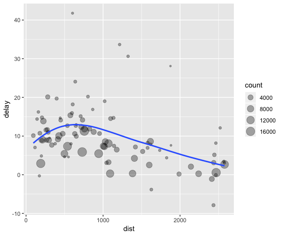
Imagine that we want to explore the relationship between the distance and average delay for each location. Using what you know about dplyr and not using pipes, you might write code like this:

by_dest <- group_by(flights, dest)
delay <- 
  summarize(
    by_dest,
    count = n(),
    dist = mean(distance, na.rm = TRUE),
    delay = mean(arr_delay, na.rm = TRUE)
  )
delay <- filter(delay, count > 20, dest != "HNL")

# It looks like delays increase with distance up to ~750 miles 
# and then decrease. Maybe as flights get longer there's more 
# ability to make up delays in the air?
ggplot(data = delay, mapping = aes(x = dist, y = delay)) +
  geom_point(aes(size = count), alpha = 1/3) +
  geom_smooth(se = FALSE)
#> `geom_smooth()` using method = 'loess' and formula 'y ~ x'

There are three steps to prepare this data:

Group flights by destination.
Summarize to compute distance, average delay, and number of flights.
Filter to remove noisy points and Honolulu airport, which is almost twice as far away as the next closest airport.

This code is a little frustrating to write because we have to give each intermediate data frame a name, even though we don’t care about it. Naming things is hard, so this slows down our analysis.

It’s better to tackle the same problem with the pipe, %>%:

delays <- 
  flights %>% 
  group_by(dest) %>% 
  summarize(
    count = n(),
    dist = mean(distance, na.rm = TRUE),
    delay = mean(arr_delay, na.rm = TRUE)
  ) %>% 
  filter(count > 20, dest != "HNL")

This focuses on the transformations, not what’s being transformed, which makes the code easier to read. You can read it as a series of imperative statements: group, then summarize, then filter. As suggested by this reading, a good way to pronounce %>% when reading code is “then”.

Behind the scenes, x %>% f(y) turns into f(x, y), and x %>% f(y) %>% g(z) turns into g(f(x, y), z) and so on. You can use the pipe to rewrite multiple operations in a way that you can read left-to-right, top-to-bottom. We’ll use piping frequently from now on because it considerably improves the readability of code, and we’ll come back to it in more detail later on.